Many statistical analysis problems involve categorical data in which observations belong to one of number of groups that have no numerical relationship between them. For example, male or female, nationality, what state a person is from, and the all time favorite of statistics textbooks, the 6 (or more) sides of a die. In this type of data, one group cannot be interpreted numerically as higher or lower than any other, but rather each group is equivalent to any other group, and membership in that group is what we’re interested in. While the 6 sides of a die have a numerical interpretation, each has an equal probability of occurring during any given roll, assuming the die is fair. Or so you would hope.
In my Categorical Data Analysis class, we explored this very assumption and looked at a paper by Karl Pearson from 1900 – On the Criterion that a Given System of Deviations from the Probable in the Case of a Correlated System of Variables is such that it Can Reasonably Be Supposed to have Arisen from Random Sampling. Very exciting, just from the title, isn’t it?? (More on that later.) In this paper, Pearson looked at a dataset (from a Professor W.F.R. Weldon) consisting of 26,306 rolls of 12 dice, and specifically “…the observed frequency of dice with 5 or 6 points…”
Seems simple enough. We can easily simulate 26,306 rolls of 12 dice and count the number of 5s or 6s. The observed data is added in, below, and we can compute the theoretical distribution of values using a Binomial Distribution in which we have 12 trials and the probability of success on any given trial is 1/3; 12 dice, count 5s or 6s.
> # simulate the 12-dice experiment
> count <- factor(replicate(26306, length(which(sample(6, 12, replace=TRUE) >= 5))),
+                 levels=0:12)
> df <- as.data.frame(table(count))
> df$Prob <- round(df$Freq/26306, 4)

> # add in the data from Pearson's paper
> df$PearsonFreq <- c(185, 1149, 3265, 5475, 6114, 5194, 3067, 1331, 403, 105, 14, 4, 0)
> df$PearsonProb <- round(df$PearsonFreq/26306, 4)

> # include the expected distribution from the Binomial Distribution
> bin <- dbinom(0:12, size = 12, prob = 1/3)
> df$BinomialFreq <- as.integer(bin*26306)
> df$BinomialProb <- round(bin,4)
> df

   count Freq   Prob PearsonFreq PearsonProb BinomialFreq BinomialProb
1      0  206 0.0078         185      0.0070          202       0.0077
2      1 1180 0.0449        1149      0.0437         1216       0.0462
3      2 3289 0.1250        3265      0.1241         3345       0.1272
4      3 5565 0.2115        5475      0.2081         5575       0.2120
5      4 6221 0.2365        6114      0.2324         6272       0.2384
6      5 5101 0.1939        5194      0.1974         5018       0.1908
7      6 2979 0.1132        3067      0.1166         2927       0.1113
8      7 1278 0.0486        1331      0.0506         1254       0.0477
9      8  375 0.0143         403      0.0153          392       0.0149
10     9   97 0.0037         105      0.0040           87       0.0033
11    10   12 0.0005          14      0.0005           13       0.0005
12    11    3 0.0001           4      0.0002            1       0.0000
13    12    0 0.0000           0      0.0000            0       0.0000
>
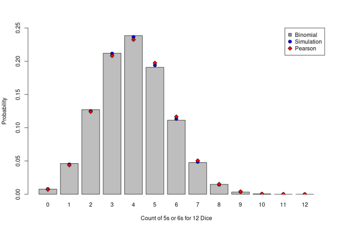
The numbers seem very close, but Pearson’s set shows consistently lower probabilities on the low side (0 through 5 counts of 5s or 6s) and consistently higher probabilities on the high side (6 through 9, and 11). Let’s look at that graphically. In the figure below, I’ve plotted the theoretical results from the Binomial Distribution as grey bars, results from my simulation as blue circles, and the probabilities from Pearson’s dice data as red diamonds. Visually the simulation seems closer to the theoretical result from the Binomial Distribution while the data from Pearson’s paper still seems to exhibit a bias. To be sure, we need to apply a statistical test.
For that statistical test, I refer back to Pearson’s paper from 1900 which actually introduced something that statisticians and data scientists use extensively – the Chi-squared Test. In fact, Pearson’s paper is considered to be one of the foundations of modern statistics and introduced the Chi-squared distribution as an alternative to the Normal Distribution which Pearson felt was being used in cases when it did not fit the data. Here I apply the Chi-squared test to these data in order evaluate the goodness of fit of the simulated or observed data to the expected distribution of observed 5s or 6s, assuming the dice are fair.
> # test the simulation for goodness of fit to the theoretical Binomial Distribution
> chisq.test(df$Freq, p=dbinom(0:12, size=12, prob=1/3))

	Chi-squared test for given probabilities

data:  df$Freq
X-squared = 17.172, df = 12, p-value = 0.1432
> # test the observed dice data
> chisq.test(df$PearsonFreq, p=dbinom(0:12, size=12, prob=1/3))

	Chi-squared test for given probabilities

data:  df$PearsonFreq
X-squared = 41.312, df = 12, p-value = 4.345e-05
The simulation seems to fit, but the observations certainly do not, given a p-value of .00004345! Clearly the observed dice are not fair based upon these observations and this would surely be of interest to a casino or anyone else depending upon the equal probability of any number occurring during any given roll.
The fascinating explanation for this experiment is actually a physical one. Consider the typical die composed of a uniform material into which the pips are drilled – in other words, material is removed to make the pips. The sides of the die are arranged such that opposite sides sum to 7 – 6 pips are opposite 1 pip, 5 pips are opposite 2 pips, and 4 pips are opposite 3 pips. As a result of this arrangement, 5 and 6 are adjacent to each other while 1 and 2 are adjacent to each other and on opposite sides to 5 and 6. This leads to the center of gravity of the die being shifted very sightly away from the sides with 5 and 6 pips leading to a very slight bias for a 5 or a 6 to land upward. Pearson’s Chi-squared test gives us the necessary tools to identify this bias – along with a very large collection of data.
26,306 actual rolls of 12 dice? It took about 1 second to simulate that on my laptop. How did they make the discoveries they did without computers?
*This blog post is based heavily on an exercise and discussion from my Categorical Data Analysis class. Seeing the application of this statistical test to identification of the physical bias that existed in the observed dice rolls inspired me to dig up Pearson’s paper and is certainly one of the best moments of my statistical training thus far. Thank you Dr. Breidt for that discussion and the inspiration.
